Getting Started

To open the swolfpy, do the following steps:

1- Open the conda command prompt.

2- Activate the environment:

conda activate swolfpy

3- Open python to run swolfpy:

python

4- Run swolfpy in python:

import swolfpy as sp
sp.swolfpy()

swolfpy

Here is the swolfpy start screen (Fig. 1). The user interface includes the following tabs:

1. Start

2. Import Process Models tab: You can change the default process models through this tab.

3. Define SWM System tab: You selected the collection and treatment processes to create a SWM system.

4. Load Project Input Data tab: You load a saved project through this tab and view/update project parameters and processes.

5. Create Scenario tab: In this tab, you can create a scenario. Scenarios can start from the collection or treatment processes.

6. LCA tab: You can perform LCA or comparative LCA in this tab.

7. Monte Carlo Simulation tab: In this tab, you can define/change uncertainty distributions for the input data and perform a Monte Carlo simulation.

8. Optimization tab: In this tab, you can minimize the selected impact category by optimizing the waste fraction or collection scheme.

If you want to create a new project, click the Start New Project button [10]. You can also load a project[11].

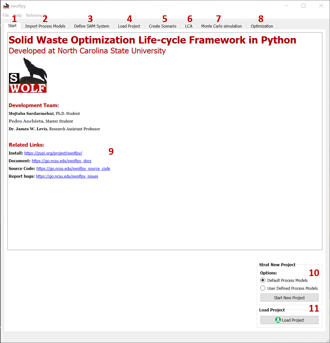
Fig. 1 Start tab

Import Process Models

If you activate the radio button for User Defined Process Models, then you will see this (Fig. 2) tab which includes three subtabs:

1. Process Models: You can select the default or user defined python models for the process models.

2. Common Data: You can change the common data file.

3. Technosphere: You can select the user defined LCI data or create a User_Technosphere database with EcoSpold2 files and connect to it.

If you have modified the default process models, then you should set them in this tab. You should select the process model from the drop-down list[4] and click the User Defined radio button[5]. Now you should click the Browse button[5] and find your python file. You can also revise the types of waste that each process models can accept through the Input Flow Type screen [6]. Don’t forget to click the Update button before changing the next process model otherwise your changes will be lost. When you are done, you should click the Import Process Models to import them and go to the next step.

Note

All the python files for the process models should be in swolfpy_processmodels directory. If you don’t know where is your installation, then do the following:

import swolfpy_processmodels
swolfpy_processmodels.__path__

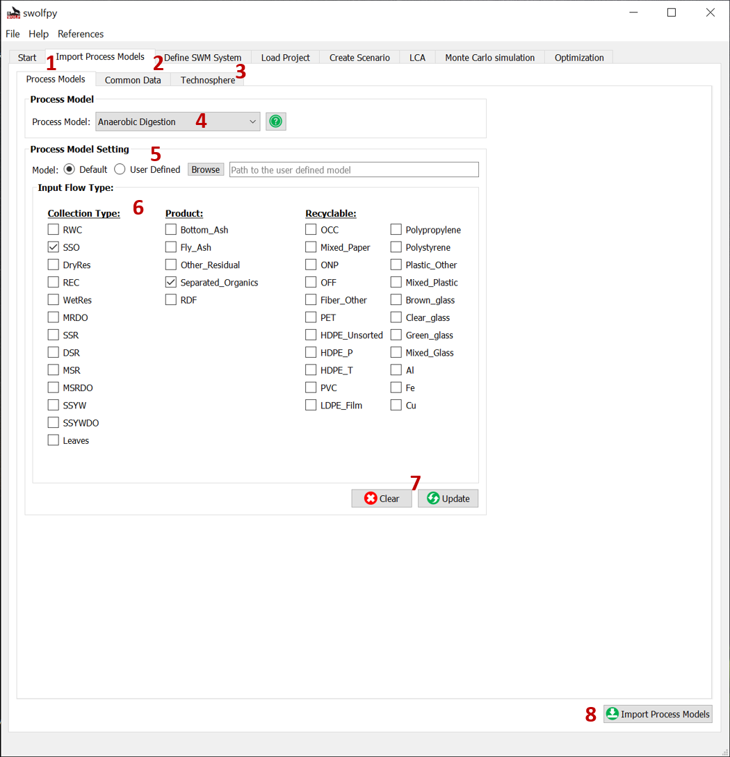
Fig. 2 Import Process Models tab.

In the Common Data subtab (Fig. 3), you can select the user defined model[1] or data[2] for the Common data.

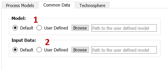
Fig. 3 Import Process Models tab: Common Data subtab.

In the Technosphere subtab (Fig. 4), you can select the user defined model[1] or LCI data [2]. You can also create a User_Technosphere database with EcoSpold2 files. In order to do that, you should select the directory that contains the EcoSpold2 files[4]. You should also add the Reference_activity_id to the Technosphere_References.csv file in the swolfpy_inputdataData directory. Then you should browse the Technosphere_References.csv [3].

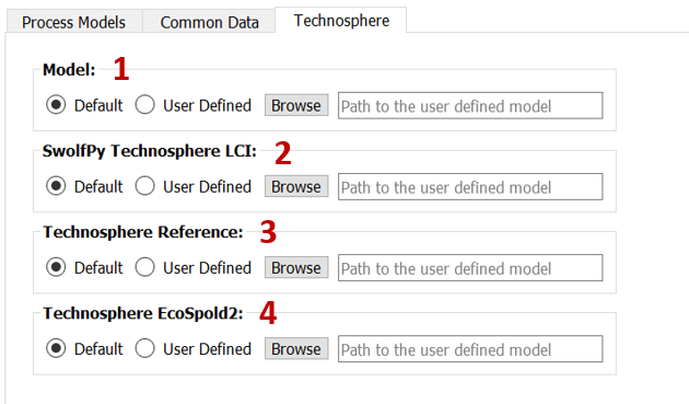
Fig. 4 Import Process Models tab: Technosphere subtab.

Define SWM System

Define Collection Processes

Note

If you are importing data, the data should be in the csv format and have the same column names as the default data files. We suggest to copy our data files and edit them to keep the structure.

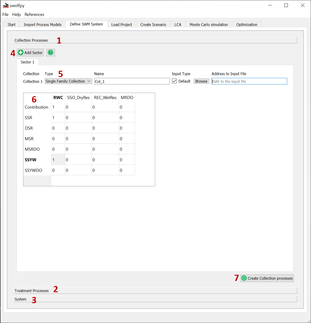
Fig. 5 Define Collection Processes for SWM system.

Define Treatment Processes

Note

If you are importing data, the data should be in the csv format and have the same column names as the default data files. We suggest to copy our data files and edit them to keep the structure.

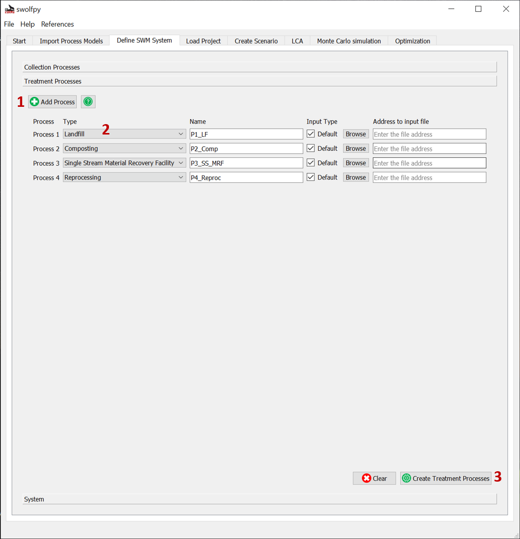
Fig. 6 Define Treatment Processes for SWM system.

Define SWM System

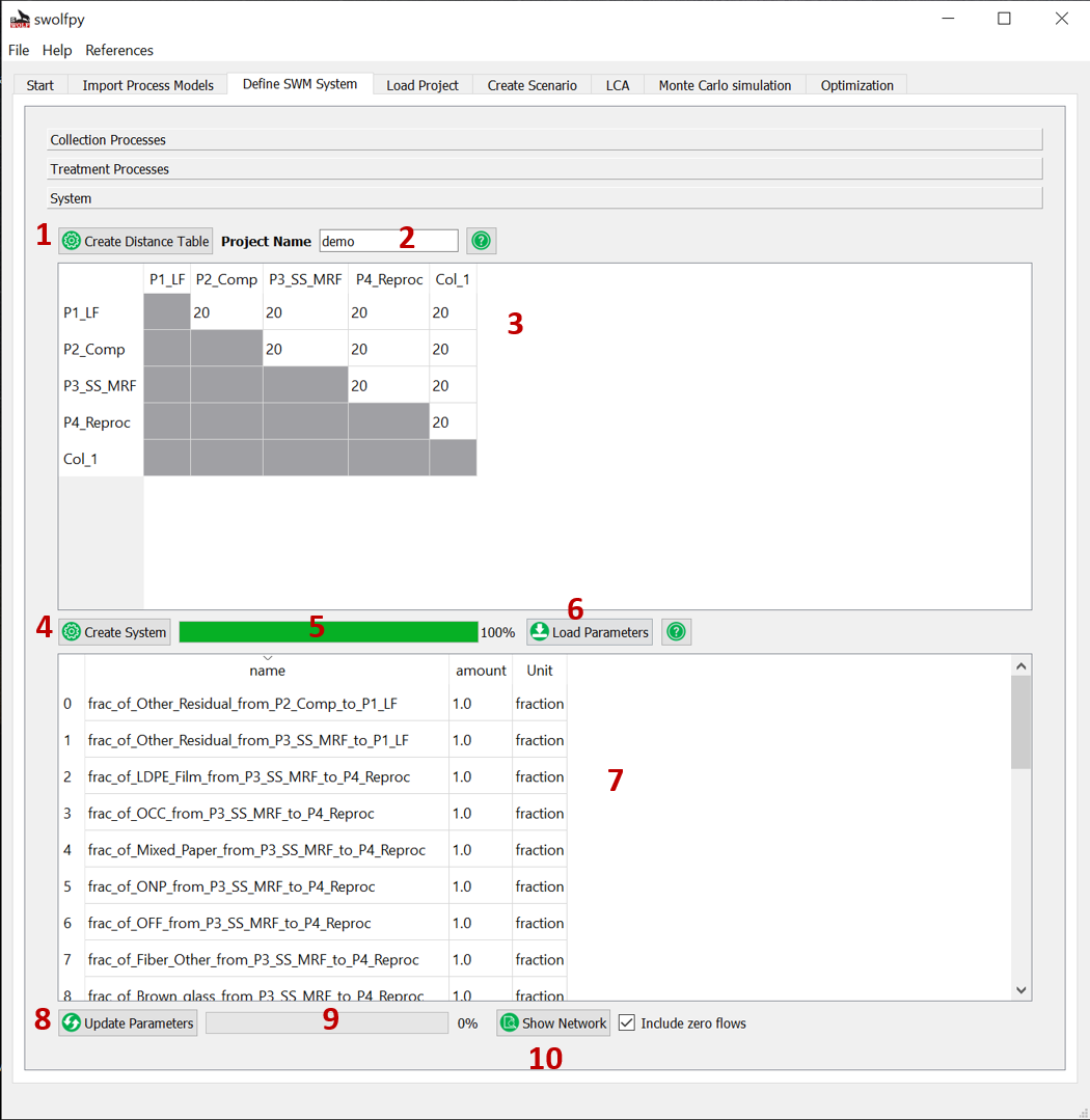
Fig. 7 Define SWM system (Distances and processes allocations).

Create Scenario

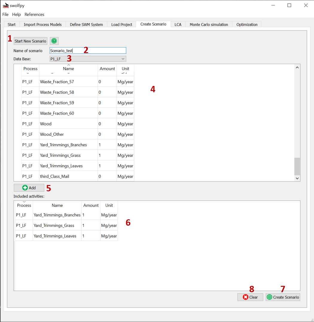
Fig. 8 Create scenario tab.

LCA

Setup LCA

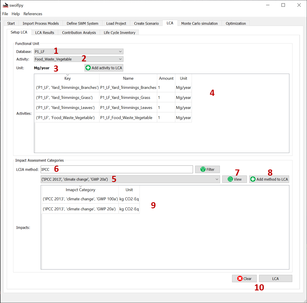
Fig. 9 Setup LCA tab (Selecting the functional units and impact assessment methods).

LCA Results

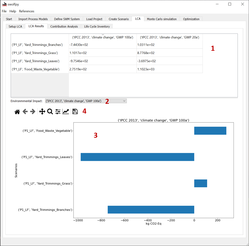
Fig. 10 LCA results tab.

Contribution Analysis

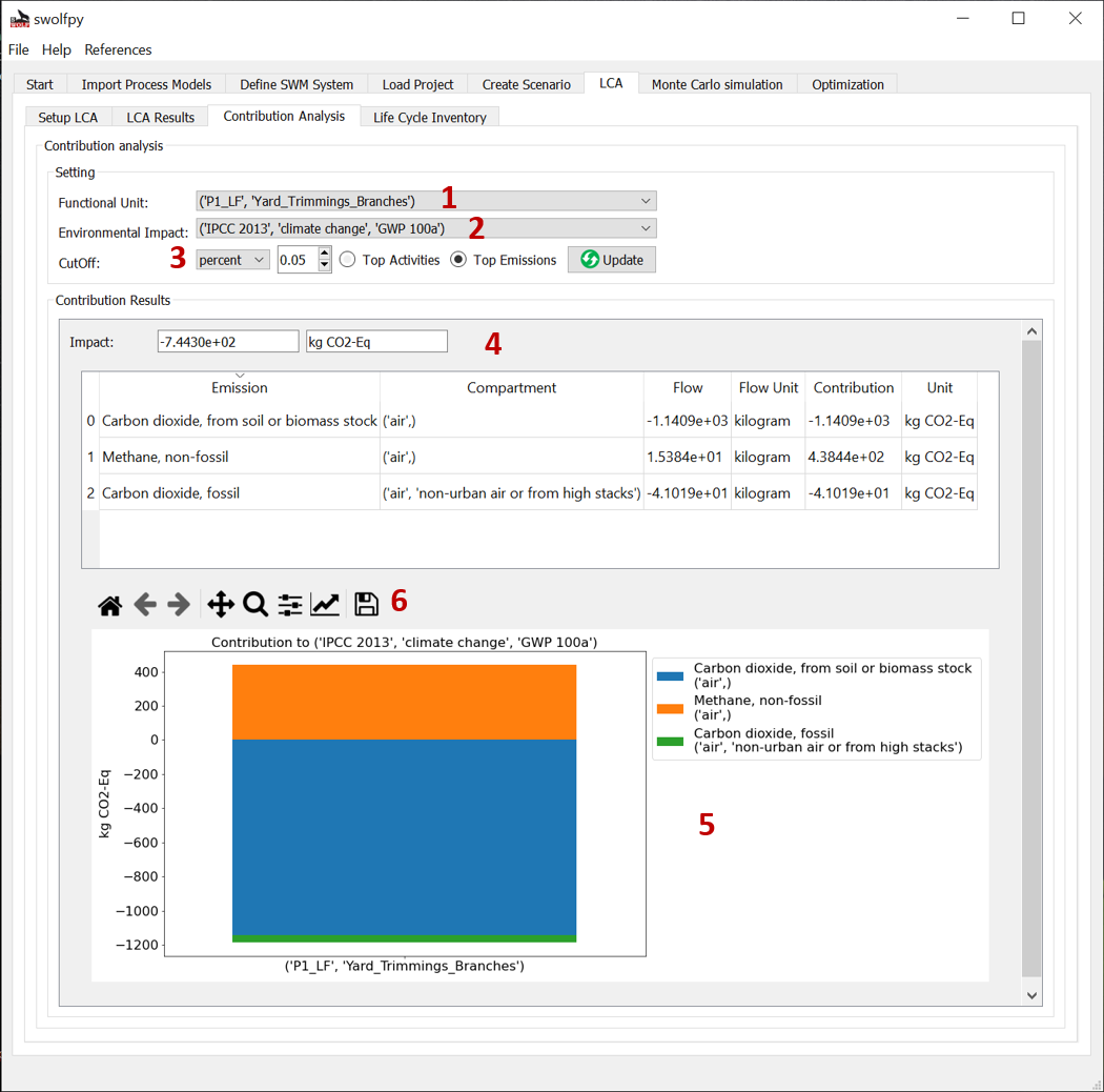
Fig. 11 Contribution analysis tab (Shows the top emissions or top activities that contribute to the selected impact).

Life Cycle Inventory

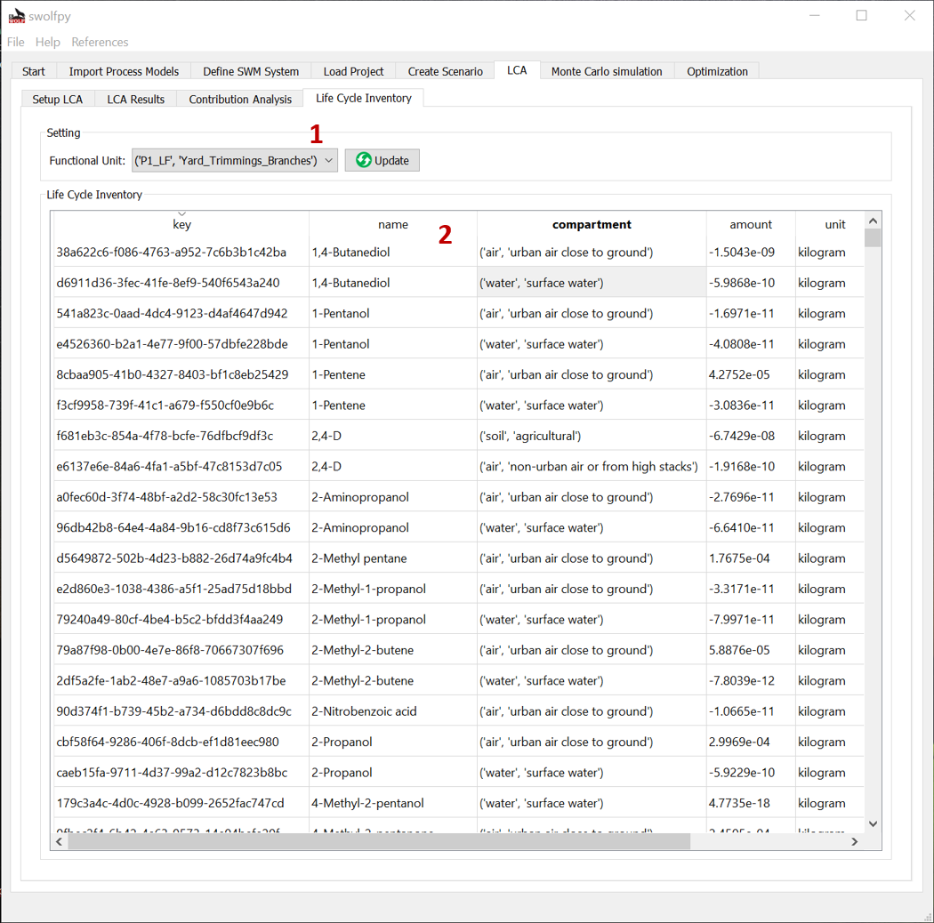
Fig. 12 LCI tab.

Monte Carlo Simulation

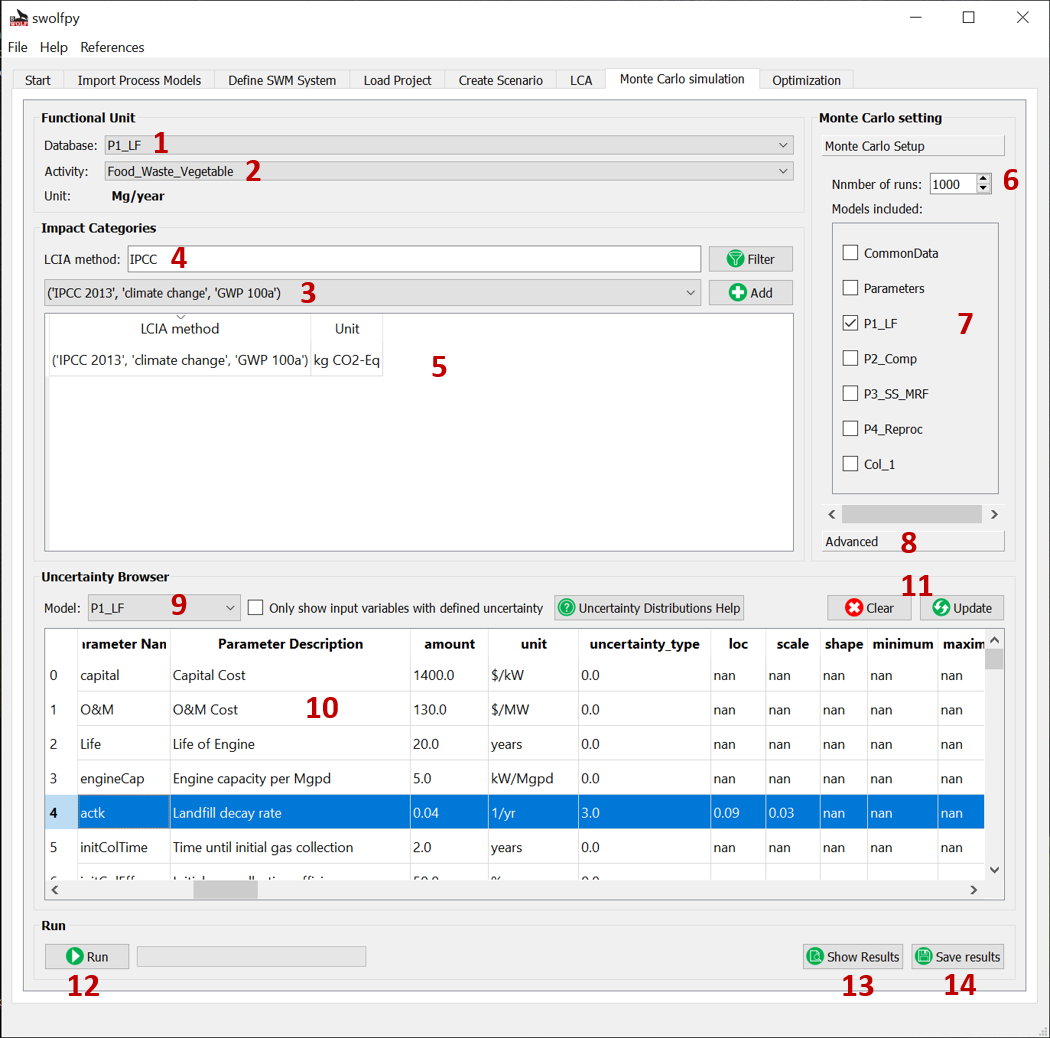
Fig. 13 Monte Carlo Simulation tab.

Monte Carlo Results

Data

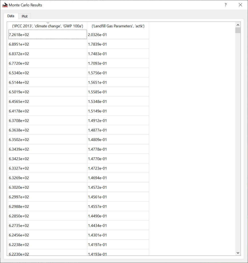
Fig. 14 Monte Carlo Simulation results window.

Plot

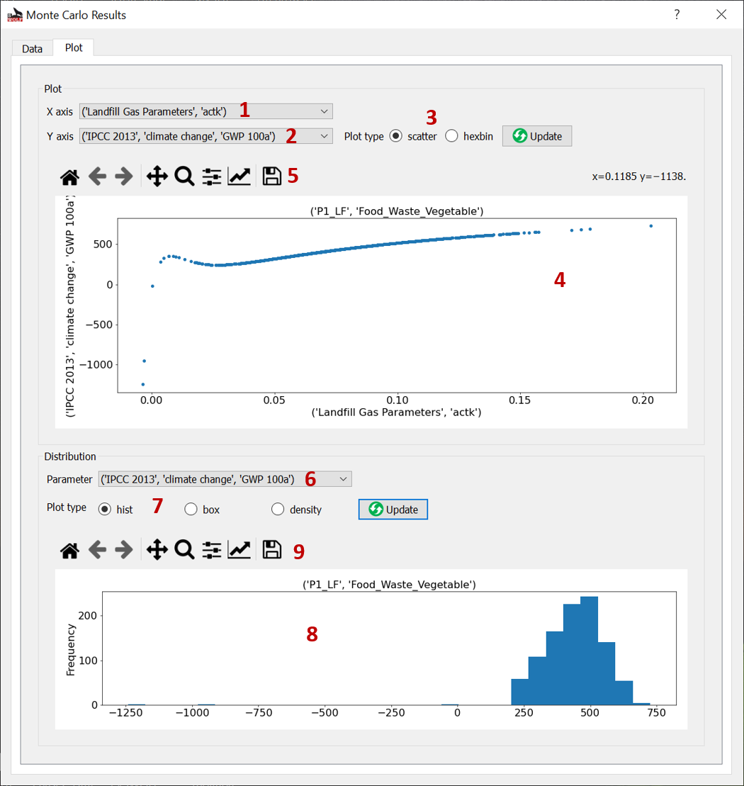
Fig. 15 Plot Monte Carlo Simulation results window.

Optimization

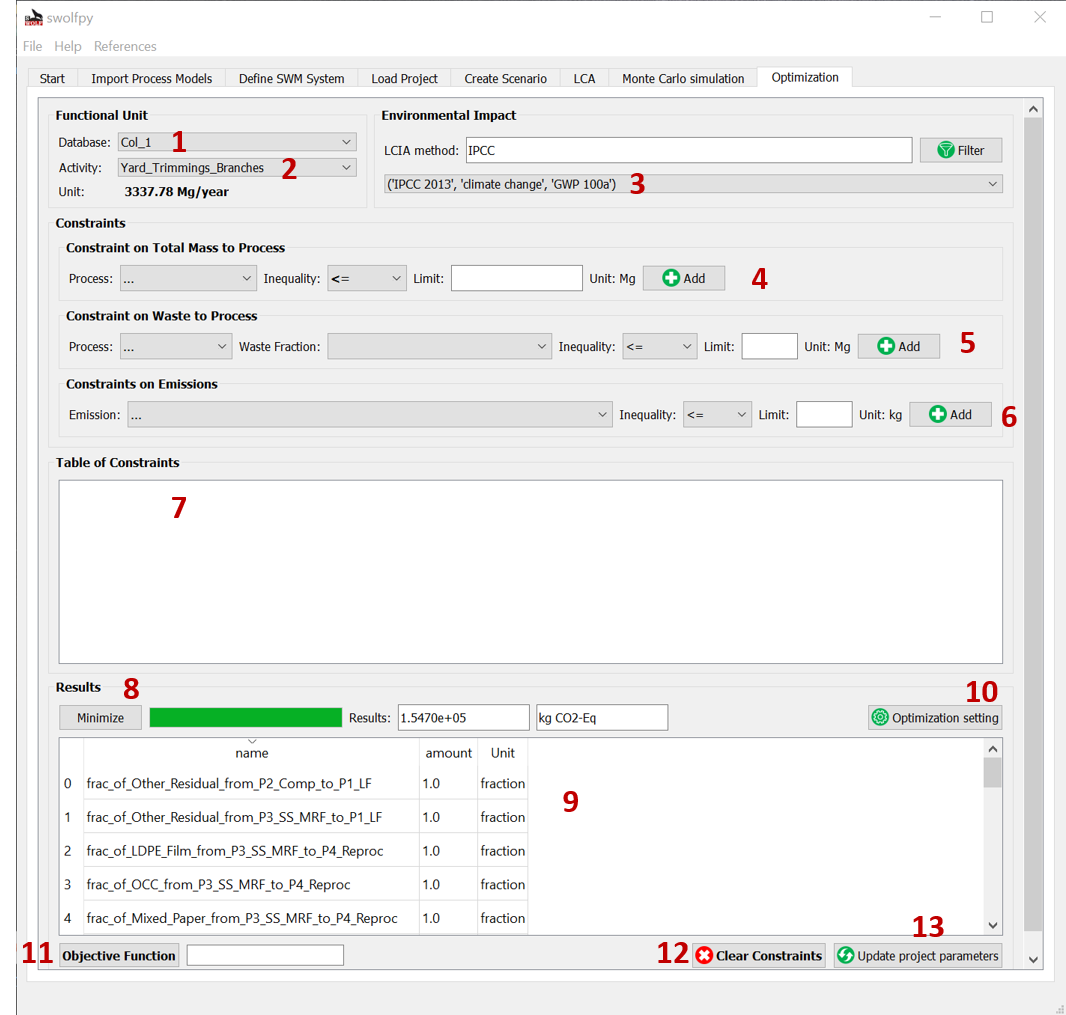
Fig. 16 Optimization tab.

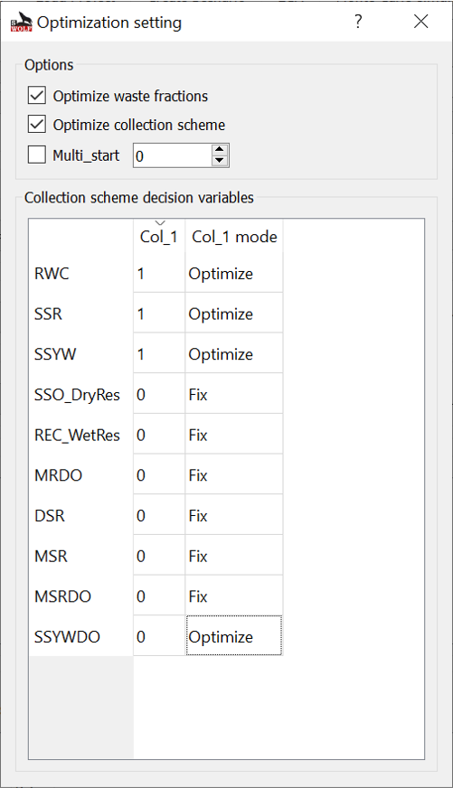
Fig. 17 Optimization setting window.

Load Project

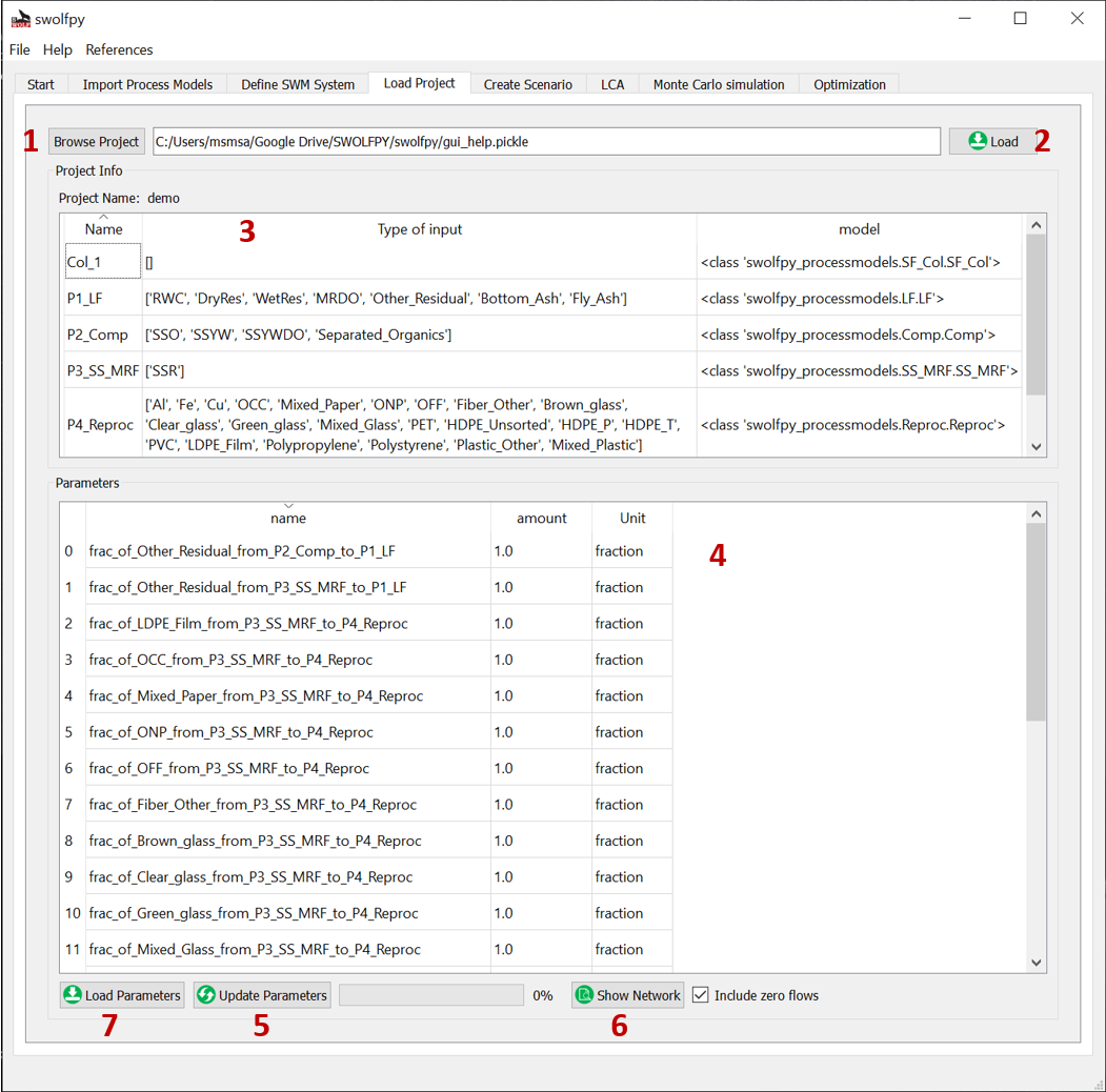
Fig. 18 Load Project tab.

Uncertainty Distribution

Tha stats_arrays package is used to define uncertain input parameters for the process models and waste materials. The table below shows the main uncertainty distributions that are currently used

Name	uncertainty_type	loc	scale	shape	minimum	maximum
Undefined	0	static value
No uncertainty	1	static value
Lognormal	2	\(\boldsymbol{\mu}\)	\(\boldsymbol{\sigma}\)		Lower bound	Upper bound
Normal	3	\(\boldsymbol{\mu}\)	\(\boldsymbol{\sigma}\)		Lower bound	Upper bound
Uniform	4				Minimum	Maximum
Triangular	5	mode			Minimum	Maximum
Discrete Uniform	7	mode			Minimum	upper bound

Guideline to define uncertainty

1. Normal distributions (ID = 3): When there is sufficient published data.

2. Triangular distribution (ID = 5): When values are based on expert opinions with a reasonable value for the mode.

3. Uniform Distribution (ID=4): When only the range is known without preference for mode.

4. Lognormal distributions (ID=2): When only one value is available or there is significant data and the value must be non-negative.

5. Discrete Uniform (ID=7): For True/False (0,1) parameters.(min=0,max=2).

Note

In Normal distribution, if the mean is too close to lower or upper bound (mostly for parameters that are fractions), use the triangular distribution.

Note

In Lognormal distribution, if the parameter is related to the emission factors, sigma should be in the range of 0.04 to 0.09 based on the quality of the data.

See also

For more information about distributions check stats_arrays website.